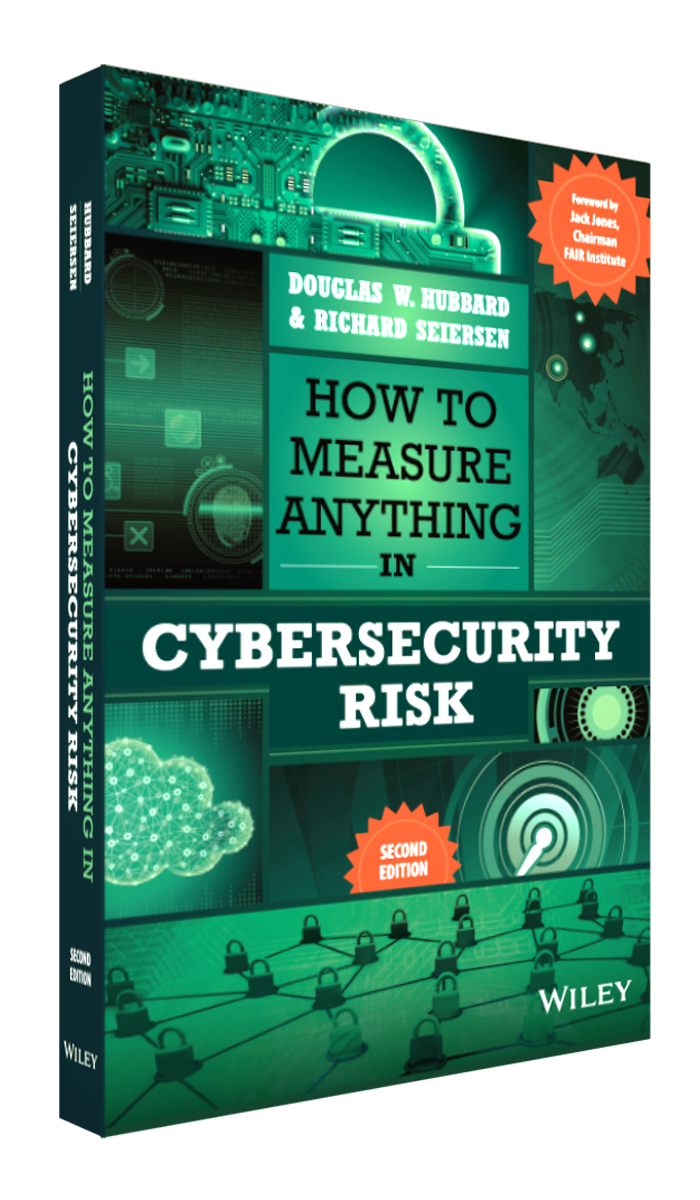
HOW TO MEASURE ANYTHING IN CYBERSECURITY RISK, 2E.
Welcome to the website for How to Measure Anything in Cybersecurity Risk, 2e. This is where readers can come to download examples mentioned in the book. These downloads include spreadsheet examples of the calculations, “Power Tools” and additional calibration exercises.
New Material For 2nd Edition!

INTERESTED IN HDR’S TRAINING?
Hubbard Decision Research offers comprehensive training in quantitative methods that decision-makers and analysts alike can apply across industries. Whether you’re looking to improve your risk analysis, forecasting, or decision-making skills, our courses provide the hands-on learning and real-world application you need to make confident, data-driven decisions.
If you are interested in learning more about Cybersecurity Risk, check out the 2-Hour, “How to Measure Anything in Cybersecurity Risk” webinar delivered by Doug Hubbard. This webinar will change how you view and measure cybersecurity risk and provide you with the tools to better protect your organization.
Do current risk assessment methods in cybersecurity work? Recent big security breaches have forced business and government to question their validity. Is there a way to fix them? How can risk even be assessed in cybersecurity?
Find the answers to these questions and more in our introduction webinar, How to Measure Anything in Cybersecurity Risk.
This two-hour webinar will change how you view cybersecurity and give you the tools to begin finding these critical answers – and better protecting your organization. Click on the button below to learn more.
Downloads for Examples and Exercises from the Book Below
Welcome to the website for How to Measure Anything in Cybersecurity Risk. This is where readers can come to download examples mentioned in the book. These downloads include spreadsheet examples of the calculations, “Power Tools” and additional calibration exercises.
Chapter 3: Simple One-for-One Substitution Example
This spreadsheet contains examples for the “one-for-one substitution” model descrbed in Chapter 3. There are three tabs. The first tab shows how tables 3.2 3.3, and 3.4 are computed in the book. The second tab shows how we add “residual” risk so that we can plot the “loss exceedance curves” (LEC) as shown in figure 3.3. Finally, there is a tab showing how multiple portfolios can be added up to to make an aggregate LEC.
Chapter 3: (Updated for 2nd Edition) Rapid Risk Audit and Simple Monte Carlo Example
As explained in Chapter 3 of How to Measure Anything in Cybersecurity Risk, the Rapid Risk Audit is a very basic, yet quantitative assessment of risks. Like qualititative methods such as the Risk Matrix, the inputs can be subjective. But although estimates may be subjective, the quantitative estimates avoid some of the errors introduced by risk matrices. This Rapid Risk Audit proposes a cause-effect taxonomy, but it could be used for any taxonomy. It will produce a total expected annual loss. But it can’t produce a probability of losing various amounts in total. For that, we need the next worksheet, the Monte Carlo simulation.
Chapter 5: (Updated for 2nd Edition) HDR Cybersecurity Survey
This was the survey conducted in 2016 for the first edition of this book. Now we are making the entire survey free for downloads.
Chapter 6: Decomposition of One-for-One Substitution Model
Chapter 7: Additional Calibration Questions
Additional calibration tests in case the tests in the book weren’t enough to get you fully calibrated.
Get the REAL calibration training here! HDR provides asynchronous training with self-paced videos so you can practice with proven methods, all while seeing your real-time calibration results on the calibrator dashboard. The data can even be used to optimize estimates on real-life problems with Team Calibrator!
Chapter 7: Expected Distribution of Calibration Answers
Chapter 8: Bayesian Threat Intel Example
This is the major data breach example from chapter 8. The tables below contain the calculations necessary to compute the table on the right from the inputs in the table on the left (in yellow).
Chapter 8: (Updated for 2nd Edition) Bayesian Multifactor Authentication
This is an example of how to use a Bayesian method to update the probability that Multifactor Authentication is working even with very limited observations.
Chapter 9: Beta Dist Example for Three Industries
Chapter 9: (Updated for 2nd Edition) Log Odds Ratios for Simple Lens and SME Aggregation
This spreadsheet has two worksheets. The first is the LOR example in Chapter 9 which provides a quick subsystem risk based on past Lens models created by HDR. The second worksheet shows how the estimates of two SMEs might be combined using a highly simplified LOR method.
Chapter 9: Log Odds Ratio Example
Appendix A: Probability Distributions in Excel
These are the calculations for Appendix A: Selected Distributions. There are several useful random distributions here that apply to a variety of different cybersecurity risks. The Binary (aka Bernoulli) produces a “1” or “0” (which can be used as “event occurred” or “event didn’t occur”). It applies to whether a security event such as a data breach occurred in the first place. The other distributions are more appropriate for types of impacts that result after an event occurs – such as a system outage, a number of records compromised, the costs of legal liabilities, and so on.


